Computational chemistry has many different tools for different goals. However, one common feature of all of them is complexity since the end product results from many years of work by numerous researchers. Luckily, you do not have to write your own from scratch; plenty of open-source codes are available now. Combine that with free computing resources such as google Colab; you can run your computational chemistry exercise in the cloud for free in no time.
Standard quantum chemistry calculations usually take too long. Also, using high-accuracy quantum chemistry might be off-limits due to the usage restrictions for free jobs in Colab (12 hours runtime and 16GB memory). Luckily, semiempirical methods provide a trade-off between accuracy and computational expense. Recently, I posted a Jupyter notebook to show how to use the xTB semiempirical code from the Grimme group in the cloud for free. This notebook was inspired by Prof. Jensen’s presentation here.
You can use condacolab to set up Rdkit and xtb (installing the packages takes a few minutes). Once that is done, starting with SMILES strings, you can calculate 3d geometries and visualize them!
%%capture
!pip install -q condacolab
import condacolab
condacolab.install()

!mamba install -c conda-forge rdkit
!mamba install -c conda-forge xtb
!pip install py3Dmol
!pip install rdkit-pypi
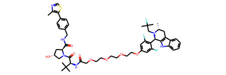
An example geometry optimization for the following PROTAC is shown in the notebook:
protac_smi = 'C[C@@H]1CC2=C(NC3=CC=CC=C23)[C@H](N1CC(C)(C)F)C1=C(F)C=C(OCCOCCOCCOCC(=O)N[C@H](C(=O)N2C[C@H(O)C[C@H]2C(=O)NCC2=CC=C(C=C2)C2=C(C)N=CS2)C(C)(C)C)C=C1F'
protac = Chem.MolFromSmiles(protac_smi)
protac

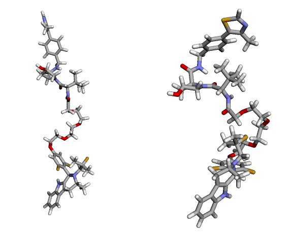
We need an initial 3D geometry for the geometry optimization with xTB. Below, the initial geometry from rdkit is shown on the left; the optimized geometry with xTB is shown on the right.

Enjoy!
Note: Unfortunately 3D geometries do not display properly in the jupyter notebook. The geometries can be seen in the original colab notebook by clicking the “Open in Colab” link.